
Here’s the latest draft chapter in Mixed Model Arts (book 1). Aggregations are another building block of data modeling, and in this chapter, I go into the fundamentals of aggregations. I haven’t seen aggregations covered very often from first principles, so hopefully this helps people understand aggregations from the ground up and avoid catastrophic mistakes. Lord knows I’ve unwittingly committed some aggregation sins, and I’m sure you have too.
I’ll give this chapter time to stew, as I’m still unsettled with this being its final state. Whenever I make edits, I’ll let you know.
Please leave a comment if you feel I’ve missed something important. If there are grammatical or similar errors, please leave a note here.
Thanks1,
Joe
In the late 1940s, the US Air Force had a serious problem: their pilots couldn’t control their planes. Crash rates were alarming, and the blame initially fell on “pilot error.” But the real culprit was a data modeling error. Designers had built cockpits based on the “average” pilot. They had aggregated the physical dimensions (height, chest, reach) of thousands of airmen to create a composite profile, a perfect standardized human. Or so they thought.
In 1950, a researcher named Gilbert Daniels put this aggregation to the test. He measured 4,000 pilots against ten of these “average” dimensions. He assumed most pilots would fit the average profile. The result? Zero. Out of 4,000 men, not a single one fell within the average range for all ten dimensions. By designing for the average, the Air Force had designed for no one. The “average man” was a mathematical ghost, an artifact of aggregation that didn’t exist in the real world.
Modeling data is more than just collecting random data and putting it in tables. Often, we want to count and aggregate our data to better understand it. While counting is technically a form of aggregation (a COUNT function), we treat them separately here because they play distinct roles in modeling. Counting confirms existence and identity, proving that specific instances exist. Aggregation focuses on summarization, combining the values of those instances into larger wholes. As the Air Force story illustrates, when aggregation is done poorly, models can describe things that do not exist.
In earlier chapters, we talked about identifying things, relating them, and establishing their grain. With those pieces in place, we can finally talk about how to count things and how those counts serve as the basis for aggregating across any form of data: tabular, text, graph, event, image, etc. Let’s begin by (re)learning to count.
What Does it Mean to Count Something?
Counting sounds obvious, and on the surface, it’s literally what it sounds like - we’re counting things. But there’s nuance to counting that requires answering some fundamental considerations about instances and identity, discrete or continuous, boundaries, context, and existence versus quantity. Let’s count the ways (pun intended).
We need to know precisely what the “thing” we’re counting is. Refer back to our discussion on instances and identity. Are we counting a row, words, or characters within a text document, an event, or pixels in an image? Two items can only be counted separately if we can tell them apart.
Does the thing exist at all (Occurrence), and if so, how many unique things exist (Cardinality)? For instance, “Does this customer exist in our system? And if so, how many orders do they have?” In data modeling, your basis for counting is strictly defined by the boundaries of the dataset you have chosen to frame.
Is what we’re counting discrete or continuous? Some things can be counted as whole units (orders, users, word count). Others can be measured continuously (e.g., temperature, pixel intensity, precipitation). A data model must specify which is which.
Counts depend on the context, scope, and conditions of the question being asked. Back to our question, “Does this customer exist in our system? And if so, how many orders do they have?” This question only makes sense within the context of “within what time range was an order placed, and under what definition of customer?”
All of this ties back to defining what “one” of something means, how many such “ones” can exist, and under what conditions. Again, counting is a type of aggregation, and arguably the simplest. Before we move to more advanced aggregates like sum or average, we need to know what “one” means. Once we understand what “one” is, we can talk about “many.” Let’s next look at how aggregation turns many small observations of “one” into a clearer view of the whole.
Aggregations: From Many to One
We now move to aggregation, the process of combining individual “ones” into larger, meaningful wholes. Aggregation allows us to perform mathematical operations, such as counting, summing, averaging (mean, mode, median), or finding the minimum or maximum, on a set of values to derive a new, summary value.
Aggregates always lose information, and every aggregation is a trade-off in the level of detail we want to capture. Whenever we aggregate, we are making two tightly coupled data modeling decisions. First, we decide which data we’re grouping or organizing. Along with this, we’re also inherently deciding what we keep and what we discard. So, aggregation is both a grouping and a filtering exercise that moves from a lower to a higher level of abstraction. For example, a handful of user events in a mobile app constitutes a session, or a collection of words constitutes a document. At a low level, either of these examples is a collection of things - user events or words.
While aggregations are commonly associated with tabular data, we can aggregate data across all forms of data. With tabular data, we group rows by a key or another attribute. Event streams fold event sequences into sessions or windows. With text data, you might compute term frequencies or aggregate word vectors into sentence embeddings. With images and video, you can pool pixels or frames into higher-level features. Although we’re working with different forms of data, the same principle applies: identify what belongs in the data, define a grain, group the data, and aggregate it.
Meaningful aggregation relies entirely on the grain of the underlying data being clearly defined. Note that I said “meaningful,” not “possible.” A database will execute an aggregation on messy data without error, but the result will be garbage. Changing the grain changes the meaning of both the grouping and the result. For example, aggregating at the event level yields different insights than aggregating at the session, document, or product level.
Grouping changes the grain and is the mechanism by which we transform the data from one grain (the input) to a coarser grain (the aggregate). Grouping, in turn, defines how instances roll up into larger entities. This could be a category, a time bucket, a cluster, a user, a region, or any other dimension we introduce into the model. Different grouping conditions produce different summaries and different interpretations of the data.
So, aggregation reduces data into a smaller, summarized form. And this new aggregated data isn’t just numbers, but also a new entity in your data model. This entity has its own attributes, identifiers, grain, and relationships. This is where data modeling becomes recursive. Data aggregates roll up into summaries, summaries become entities, and these entities might themselves be aggregated further. Many become one, and these new “ones” are now available to become part of an even larger whole.
Structural Principles of (Safe) Aggregation
Aggregation seems simple enough, but be careful not to treat it lightly. Poorly constructed aggregations have ruined many data models. Some structural rules and constraints determine whether an aggregation is safe and valid. These rules hold across all forms of data: tables, documents, graphs, events, vectors, images, and more. If these rules aren’t respected, aggregation produces contradictions, double counting, or mathematically invalid results. Remember, data modeling is about making data that’s useful and trustworthy.
Identify and Align the Data Grain
As established in the previous chapter, structuring the right data model means organizing data at the appropriate level for its intended use case. The most fundamental concept governing the data model’s aggregation structure is the data’s grain.
Data can only be successfully aggregated when it shares the same grain. Conversely, if you combine different data with mismatched grains or choose the wrong grain for an aggregation, the result is structurally unsound. Aggregation is meaningful only when all aggregated items share the same, defined grain. Suppose you combine different datasets with mismatched grains and meanings, for example, user event sessions for a mobile game combined with IOT readings of hummingbird flight patterns. In that case, the result is silly at best and structurally unsound by default. Your data model must ensure that each instance has a defined grain and that every aggregate operates on instances of that grain. Every change in grain due to aggregation must be explicit and never accidental. Violations here are the root cause of most incorrect aggregates.
Let’s look at some of the problems with mismatched grains and incorrect aggregates.
- Double counting. A low-grain item (such as a transaction) is mistakenly combined with a high-grain item (such as a customer) without a proper many-to-one relationship, causing the high-grain item to be counted multiple times.
- Confusing aggregates. Aggregating a high-grain item (like a session) with a low-grain item (like a minute-by-minute heartbeat ping) can obscure or average out the critical detail contained in the lower-grain data.
- Ambiguous interpretation. The resulting metric has no clear, traceable definition, making it impossible to validate or trust. For instance, combining “daily unique visitors” (grain: day-user) with “page views” (grain: page view event) without proper grouping will yield an aggregation that is neither an accurate count of users nor a precise count of views.
Now that we understand the problems, let’s look at some rules to guarantee grain integrity. A robust and trustworthy data model must enforce strict rules that aggregation operations remain consistent and accurate. The model must explicitly guarantee the following principles of sound grain management.
- Each instance has a defined grain. Every table or dataset must have its grain explicitly documented and understood by all users. This eliminates ambiguity about what each data instance represents.
- Every aggregate operates on instances of that grain. When calculating a sum, average, or count, the operation must be performed only on a set of records that share the same grain as the final metric. If an aggregate requires a change in grain (e.g., counting daily sessions to get monthly unique users), the change must be an explicit, deliberate operation (e.g., using COUNT(DISTINCT user_id)).
- Grain changes are explicit, never accidental. Any transformation in the aggregation process that alters the underlying grain, such as joining two tables or performing a grouping operation, must be a conscious, documented step. Grain alteration should never be a side effect of a poorly constructed query or an ill-conceived join.
Violations here are the root cause of most incorrect aggregates. Inaccurate revenue figures, skewed user metrics, and misleading performance reports can almost always be traced back to a failure to respect and manage the data’s fundamental grain. Maintaining grain integrity is not merely a best practice but a prerequisite for generating useful and actionable data models.
Grouping Like Items
Once you’ve established the correct grain of a dataset, the items must be grouped. Grouping data into a specific shape or form implies the intent to aggregate it. An area I see people mess up often is working with disjoint versus overlapping datasets. Disjointness means that every single instance in a dataset belongs to exactly one group.
Think of it as “mutually exclusive” buckets. When you drop a data point into a group, it cannot exist in any other group at the same time.
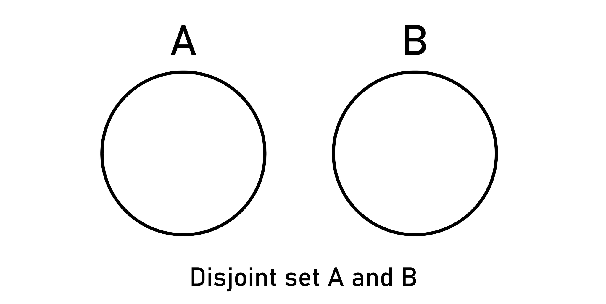
Figure x-y: Disjoint sets A and B
If your groups are disjoint, you can safely sum, count, or average them, and the total will match the total of your raw data. On the other hand, if your groups overlap, a single instance appears in multiple groups. If you aggregate on these groups, you’ll aggregate that instance numerous times. It might lead to double-counting the instance or inflated sums.
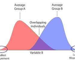
Figure x-y: Overlapping groups A and B
Here is an e-commerce example contrasting disjoint (safe) vs. overlapping (unsafe) grouping, using Order Revenue as the metric. Imagine your total revenue for the day is $9000 from 100 orders. In the disjoint (safe) scenario, every order is shipped to exactly one destination. Let’s say two orders for $4000 each, going to New York, and another order for $1000 is bound for California. Let’s group our aggregation by US state. Because these groups are disjoint, we can safely sum the orders for each state (New York = $8000, California = $1000, Total = $9000), and the math works perfectly.
Now, let’s look at the overlapping (unsafe) approach, where an order might contain items from multiple categories (or a single item that spans multiple categories). If we group by Product Category, we’ll get some very strange results. For example, we sell a smartwatch which is tagged under three categories: Electronics, Fitness, and Accessories. A customer buys a smartwatch for $300. If we group by Product Category, our query will return Electronics, Fitness, and Accessories, each with revenue of $300. This is because the Product Category results have three rows for the same smartwatch. Now, let’s sum the revenue across all categories to find “Total Daily Sales,” which, in this case, counts the sale of the watch three times, adding $900 and a quantity of 3 to our report, when we really only sold $300 and one item.
The takeaway is that disjointness enables clean aggregations, such as counts and sums. Pay close attention to whether your groups are disjoint or overlapping. Make sure each instance contributes exactly once, given the grain of your data.
Additivity (or Lack Thereof) and Nulls
Now that you’ve identified what you’re modeling, established its grain, and grouped the data, it’s time to determine how you’ll aggregate it. The behavior of an aggregation depends entirely on the mathematical properties of the data itself.
When aggregating, the measures you use generally fall into three buckets:
- Additive quantities: These can be aggregated across all dimensions. Common examples include transactional counts, total sales amounts, or quantity sold. You can sum these by day, store, region, or customer without losing meaning.
- Semi-additive quantities: These can be aggregated across some dimensions, but not others, usually time. A classic example is a bank account balance or current temperature. It makes sense to sum all customers’ balances to get today’s total bank liability, but it makes no sense to sum a customer’s balance from yesterday and today.
- Non-additive quantities: These cannot be directly aggregated at all. This category includes averages, ratios, and percentages (e.g., profit margins). To aggregate a non-additive quantity, you must usually break it down into its additive components (numerator and denominator) and calculate the result dynamically at query time.
There’s also the pesky issue of nulls, or the absence of data. Null values are a common source of logic errors in aggregation, particularly in tabular data aggregations. Let’s look at some examples. In SQL, aggregate functions like AVG() generally ignore NULL values rather than treating them as zero. This changes the denominator of your calculation. For example, imagine a column of test scores: 10, NULL, 20. If this is implicitly calculated, as in the case of (10 + 20) / 2 = 15, the NULL is skipped entirely. In another case, NULL might represent a score of zero, and the math should be (10 + 0 + 20) / 3 = 10. Suppose you are aggregating data where missing values should be treated as zero (or some other default). In that case, you must explicitly handle this transformation upstream or use SQL functions such as COALESCE to convert them before aggregation. Unfortunately, these problems are very easy to overlook, so double-check your code and make sure you’re properly handling nulls.
Decomposability and Closure
Data is very rarely neatly ordered out of the gate. You’ll often break it apart and sort the data in various ways. When aggregating data, ensure the aggregation preserves its meaning. A quantity is decomposable if you can break it into parts, aggregate the parts, and recombine them without changing the meaning.
This is especially important when aggregating across distributed systems such as Spark, BigQuery, or Snowflake. If a measure is decomposable, the database engine can calculate partial results on different servers and combine them at the end.
Let’s look at the “safe” operations. Aggregations such as COUNTS, SUMS, MINS, and MAXES are decomposable. As a simple example, you can sum records on Server A, sum other records on Server B, and sum the results on a Main Server to get the global total.